MFL NDE Scanner

Objective

Reinforced-concrete bridge decks and girders depend on steel reinforcement — longitudinal rebar tied to transverse stirrups — buried under several centimeters of concrete cover. Years of moisture and de-icing salt drive chloride-induced corrosion that eats the steel from the inside, shrinking its cross-section and the structure's load capacity long before anything shows at the surface. The aim of this research was to find and map that hidden section loss non-destructively, so inspectors could pinpoint exactly where a structure needs reinforcement.

How Magnetic Flux Leakage Works

Magnetic flux leakage (MFL) drives the embedded steel toward magnetic saturation with a powerful magnet carried over the surface. Where the bar is intact the flux stays inside the steel; where corrosion has removed material, that flux is forced out into the surrounding space and “leaks.” A sensor riding behind the magnet measures the leakage field, and the resulting anomaly marks the defect.

Two physical effects dominate the measurement. The periodic transverse stirrups each produce their own strong, repeating signature that has to be separated from genuine defects, and the concrete cover acts as lift-off — the farther the steel sits from the sensor, the weaker and broader every signal becomes.

Interactive Simulator

The model below is an interactive recreation of that measurement. The 3D view shows the concrete member (translucent), the main bar, the transverse stirrups, and the two-magnet scanner with its sensor; the trace beneath it is the MFL amplitude the sensor would record along the length of the member.

• Pitting Corrosion Level grows the defect (red) and its inverted-polarity spike in the trace.
• Transverse Bar Spacing re-lays the stirrups and reshapes the periodic background signal.
• Concrete Cover lifts the scanner away from the steel — watch every feature attenuate and spread as cover increases.
• Scanner Position (amber line) marks where the head currently sits over the scan.

Drag inside the 3D view to orbit the camera; scroll to zoom.

Open full screen →

Mathematical Model of the MFL Signal

The interactive model above is built directly on the equations below. A localized disruption of a fully magnetized reinforcing bar — pitting corrosion or a wire fracture — behaves as a localized magnetic dipole, and a differential sensor payload (a Hall-effect array sitting in a magnetic null) passing through its stray field registers a distinct bipolar signature.

1. The Bipolar Defect Model (Gaussian Derivative)

The spatial flux-leakage signal $B(x)$ from a single localized defect along the scanning axis $x$ is modeled well by the first derivative of a Gaussian:

• $B(x)$ — measured magnetic flux density (signal amplitude) at position $x$.
• $A$ — peak amplitude factor, proportional to the volume of cross-sectional loss (more corrosion → larger $A$).
• $x_c$ — center of the defect; the form guarantees $B(x_c) = 0$, reflecting purely horizontal flux directly over the dipole.
• $w$ — spatial width, setting the spread of the signal; it tracks both the physical width of the flaw and the sensor's distance from the rebar.

The negative sign is a convention fixing the polarity of the leading versus trailing edge as the sensor approaches the dipole.

2. Concrete Cover & Lift-Off Attenuation

In concrete the sensor cannot sit on the steel; the field must propagate through the cover, the NDE “lift-off” $h$. A dipole field diverges rapidly in three dimensions, so the amplitude attenuates sharply with cover — modeled by an inverse power law:

• $A(h)$ — amplitude measured at the concrete surface.
• $A_0$ — baseline amplitude with the sensor touching the defect.
• $h$ — concrete cover depth (lift-off).
• $n$ — decay exponent. A pure point dipole gives $n = 3$; for finite defects in long cylindrical rebar, empirical data usually places $n$ between $1.5$ and $2.5$.

The width $w$ also grows with $h$: as the sensor moves away the signal becomes both weaker and spatially broader, degrading resolution and blurring the defect's edges.

3. Superposition & Reinforcement Interference

In a real section the defect is rarely isolated — the sensor also picks up the stray fields of the transverse reinforcement (stirrups or ties). Because magnetic fields superpose linearly, the total signal $S_{\text{total}}(x)$ is the algebraic sum of the defect signal and the signals from the $N$ surrounding transverse bars:

Expanding with the Gaussian-derivative model gives the full signal for a congested section:

• $A_d, x_d, w_d$ — amplitude, center, and width of the main defect.
• $A_s, w_s$ — amplitude and width of the transverse stirrups.
• $x_i$ — center of the $i$-th stirrup.

Why this is hard: the defect term may be a sharp, high-amplitude pulse (small $w_d$), but the sum of $N$ stirrups builds a complex, continuously undulating baseline. Separating the two is the core data-processing problem — the evaluation software has to apply spatial-frequency filtering or differential subtraction to isolate $B_{\text{defect}}(x)$ from $\sum B_{\text{stirrup}_i}(x)$.

Reading the Signal

Pulling the defect out of that stirrup background is the practical crux of the method, and it is what the evaluation software exists to do. In the field, post-processing applied spatial-frequency filtering and differential subtraction to isolate the defect regions from full scans, producing the location maps used to decide where a structure should be reinforced.

Sensor Payload & Analog Front-End

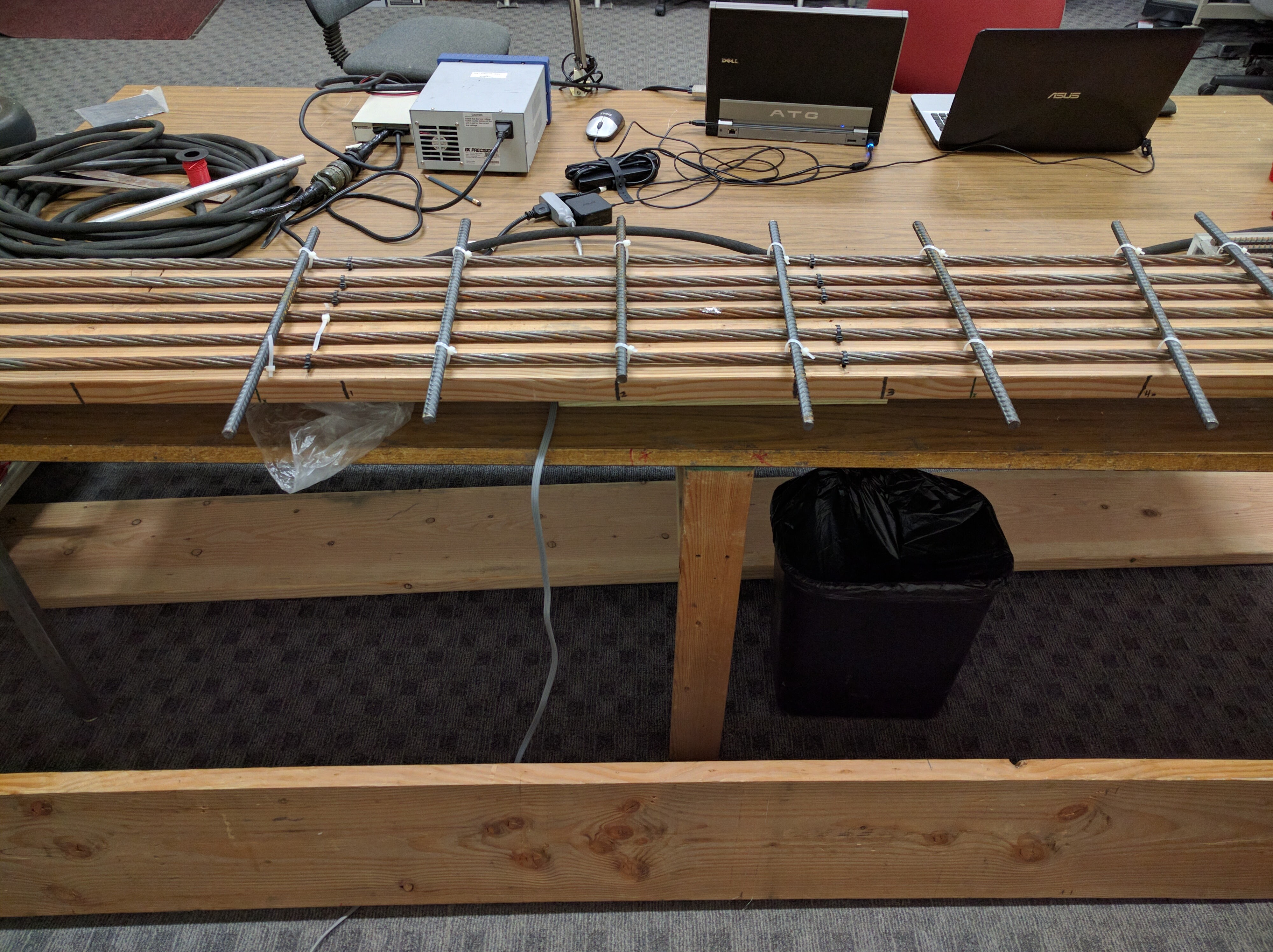
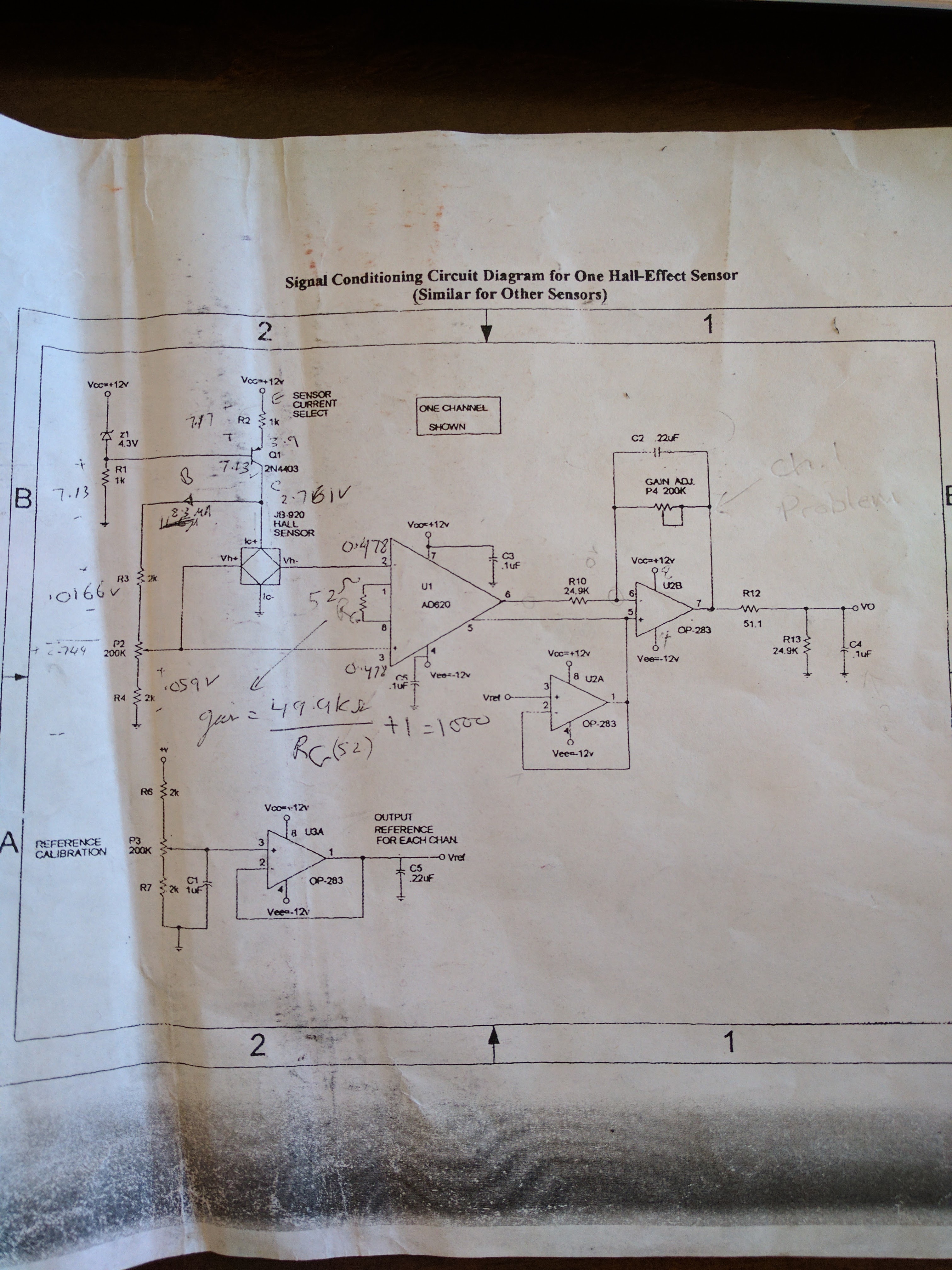
The payload carried Hall-effect sensors that picked up the leakage field along three axes, and each channel had its own analog front-end. An early build (the printed schematic) ran an A3920 Hall sensor into an AD620 instrumentation amplifier at a gain near 1000, followed by OP-283 conditioning stages. Alongside it, the whiteboard works through the active second-order Butterworth low-pass — a clean √2-damped response at a gain of 100 — whose topology and component values carried into the board revision further down. The bench shot shows a steel-strand specimen and the acquisition laptops mid-test.

Tap any image to open it full size.

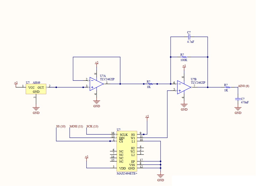
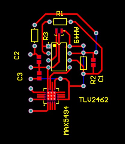
Digital Design & PCB Layout

A later revision moved the gain into the digital domain and realized the whiteboard filter directly. The channel was rebuilt around an AH49 Hall sensor and a TLV2462 rail-to-rail op-amp implementing the 4.7 nF / 100 kΩ, gain-of-100 stage from the derivation above, with a MAX5494 SPI digital potentiometer setting the gain — so a microcontroller could calibrate each channel in software before the signal reached the ADC input (AIN0). The board below is the routed single-channel version of that design.

Further Reading

Magnetic Flux Leakage for NDE